We pruned DeepSeek-V4-Flash’s experts from 256 to 128 per layer, shrinking the 167 GB checkpoint to 82 GB, and ran it at 17 tok/s with stock vLLM on a single DGX Spark. The whole pipeline, including calibration, ran on that same 128 GB machine, which cannot hold the full model.
- Model: https://huggingface.co/ludo-tech/DeepSeek-V4-Flash-REAP-145B-A13B
- Method: expert pruning with REAP (Cerebras, ICLR 2026)
- Along the way, calibrating on English only made the model answer Japanese questions in Chinese. That story is included below.
1. Introduction
About DeepSeek-V4-Flash
DeepSeek-V4-Flash is an MIT-licensed Mixture of Experts (MoE) LLM from DeepSeek. A preview came out first, and the official 0731 release followed on July 31. The 0731 release improved substantially on agentic benchmarks (Terminal Bench 2.1 went from 61.8 to 82.7), and it is the version this article is about.
The model has 304B parameters in total, but about 20B of that is the MTP head used for speculative decoding, so the main body is 284B. Active parameters per token are 13B. Each layer has 256 routed experts, and 6 are selected per token. The distributed checkpoint stores experts in FP4 and attention in FP8, and it still comes to 167 GB.
With 13B active, this is a model that should run at practical speed locally, if only it fit.
The standard setup is two DGX Sparks. I wanted one.
On X, the standard recipe for running DeepSeek-V4-Flash locally has become “connect two DGX Sparks for 256 GB”. The full 167 GB fits with room to spare for the KV cache. It is the proper way to do it.
But I wanted to run it on the one machine I have: a GB10 with 128 GB of unified memory and a 4 TB NVMe. Buying a second one would solve the problem, but my underlying complaint was that few models make a 128 GB machine feel worthwhile on its own. The well-known models that run on a single Spark are things like Qwen3.8-27B and Qwen3.6-35B, which have too few parameters to be fully satisfying in quality (they are still very good!). V4 Flash is fast at 13B active and high quality, and the only problem is that it is 39 GB too big. If I could deal with those 39 GB, it might be the best model that runs on a single Spark. That was the motivation.
The obvious answer would be quantization, but this model is already FP4/FP8. There is almost nothing left to squeeze, and the quality impact of squeezing further is unpredictable.
So I turned to the remaining option: expert pruning. An MoE only uses 6 of 256 experts per token, so deleting the unused experts outright reduces size while leaving every remaining tensor byte-for-byte identical.
Goals
- Reduce the number of experts per layer, K, from 256 to 128, bringing the checkpoint to 82 GB
- Run it on stock vLLM (no patches)
- Reach at least 17 tok/s decode as a practical speed
- Keep Japanese usable
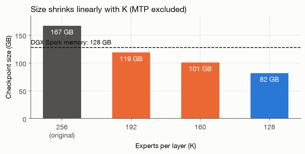
Why K=128 is explained in section 4. The short version: it is a constraint of vLLM’s router kernel.
2. REAP, the MoE pruning method
Why “drop the experts that are selected least often” is not enough
The simplest approach is to run calibration text through the model and drop experts starting from the least frequently selected. If that worked, REAP would be unnecessary. When I actually counted, two reasons it does not work became visible.
Reason 1: a lot of tokens still flow to the experts you would drop.
The figure below sorts each layer’s 256 experts by how often they were used and plots what fraction of routing the top N experts account for. Even keeping half, 128 experts, covers only 60 to 80 percent. The remaining 20 to 40 percent of tokens go to experts on the “drop” side.
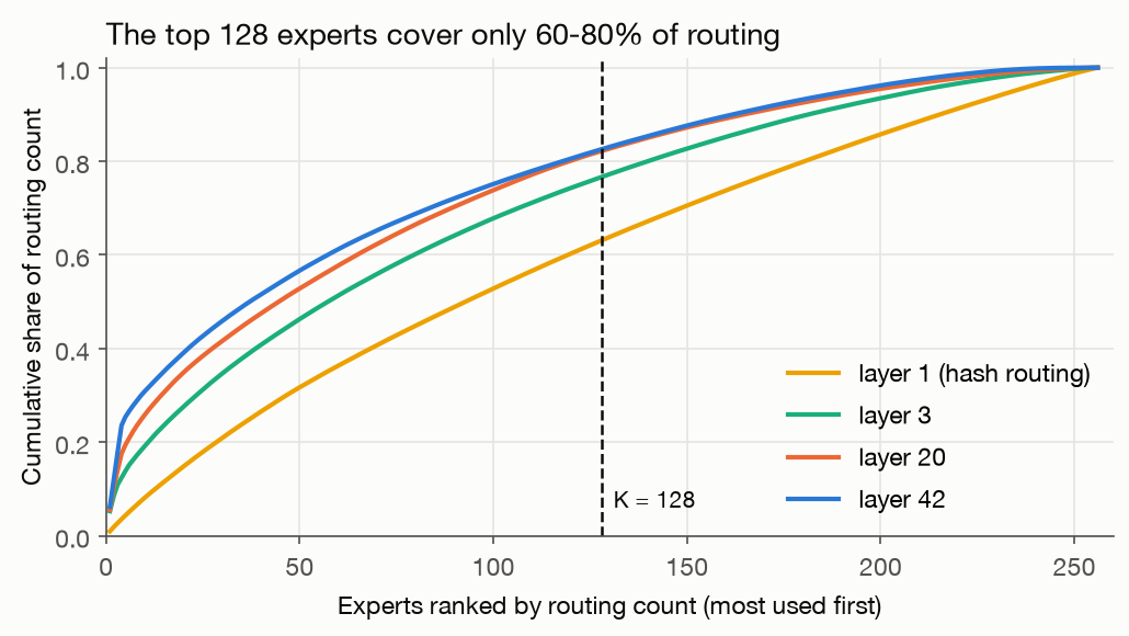
In other words, this is not a matter of dropping only the “rarely used” experts. To get down to 128, you have to drop experts that are used a fair amount, and the criterion for which ones matters. Layers 0 to 2 have a special routing mechanism (section 4) with an almost flat distribution, which makes it matter even more.
Reason 2: “called often” and “contributing a lot” are different things.
An expert’s output is multiplied by the router weight before being added to the residual stream. If an expert is called often but returns a small output with a small weight each time, dropping it changes little. Conversely, an expert that is called rarely but returns a large output with a large weight when it is called will hurt when dropped. Counting alone drops the latter.
The REAP score
REAP (Router-weighted Expert Activation Pruning) is a one-shot MoE compression method proposed in a paper from Cerebras. The paper is titled “Why Pruning Prevails for One-Shot MoE Compression”, and its claim is that pruning experts preserves quality better than merging them.
The score for expert is:
- : the weight the router actually gave expert for that token (normalized after top-k)
- : the output vector of expert
So it is “router weight × output norm”: the average magnitude that the expert actually adds into the residual stream. It measures contribution, not count. The implementation just wraps each layer’s expert block and accumulates and per token.
w = top_k_weights[tok, pos].float()
norms = expert_out.float().norm(dim=-1)
self.sum_wnorm[e] += (w * norms).sum()
self.count[e] += tok.numel()
# S_e = sum_wnorm / count
How much does the selection change between count and REAP?
The next figure scatters the experts of layer 20 with routing count on the x-axis and REAP score on the y-axis. The 128 kept by REAP (blue and green) are cut by a horizontal score threshold, and the 128 kept by count (blue and orange) are cut by a vertical line.
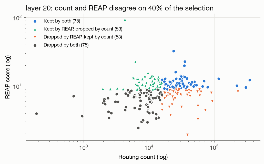
The two disagree on 53 experts, which is 40 percent of 128. The average across all 43 layers was 51. Choosing by count versus by REAP is not “roughly the same”; you get a model that is nearly half different.
The interesting part is the green triangles (kept by REAP, dropped by count) clustered around 10,000 calls: experts that are selected a moderate amount but contribute heavily when they are. These are the specialists. Functions like Japanese, which are a minority of the corpus overall but essential for their tokens, are likely carried here.
3. Challenge 1: calibrating a 167 GB model on a 128 GB machine
The whole model does not fit in memory
To collect REAP scores, you have to run text through the unpruned model. But the unpruned model is 167 GB and does not fit on the Spark. Chicken and egg.
Renting an H100 in the cloud for a few hours would solve this. But the point of this article is to do everything on a single Spark, so I looked for a way to do it there.
Layer-streaming inference
A Transformer just passes through its layers in order, so all layers do not need to be in memory at once. Load one layer’s weights, run every sample through that layer, write the outputs to disk, load the next layer. Repeat 43 times and you get the same forward pass as the full model.
flowchart LR
    CK[(safetensors
167 GB, NVMe)]
    MM[(hidden stream memmap
512 × 2048 × 4 × 4096 bf16
= 34 GB, NVMe)]
    subgraph GPU["GPU memory (one layer only)"]
        DQ[FP4/FP8 → bf16
dequantize] --> L[DeepseekV4DecoderLayer i]
        L --> OBS[REAP observer
sum_wnorm, count]
    end
    CK -- raw tensors of layer i --> DQ
    MM -- read --> L
    L -- write back --> MM
    OBS --> PT[obs/layer_i.pt]
The key points:
- The hidden state lives on disk as a memmap of shape
[N, L, hc_mult, D]. V4 uses mHC (Manifold-Constrained Hyper-Connections), so there are 4 residual streams, givinghc_mult=4andD=4096. With 512 samples × 2048 tokens that is 34 GB. This is where the 4 TB NVMe earns its keep - Each layer reads raw tensors from safetensors, dequantizes FP4 (block 32, e8m0 scale) and FP8 (block 128×128) back to bf16, and assembles a
DeepseekV4DecoderLayerfromtransformers. Not having to write attention or mHC myself means that if the transformers implementation is correct, mine is too - Only the expert block is swapped for a REAP wrapper that collects statistics
- After each layer finishes, it writes
obs/layer_i.ptso the run can resume midway
It took about 7 minutes per layer, roughly 5 hours for 43 layers. There is no room for parallelism, but it finishes while you sleep.
How to make sure a home-made harness is correct
Since I am assembling layers by hand, a mistake anywhere in attention masks or RoPE handling would turn the REAP statistics into statistics of a broken model. I verified in two stages.
- With a small synthetic checkpoint (same architecture, small dimensions), a unit test confirms that the full-model logits match the layer-streaming logits
- On the real machine, apply the LM head after the last layer, compute perplexity on held-out samples, and use that as a gate. It was 3.14 for the English-only calibration and 4.73 for the Japanese mix (higher because Japanese Wikipedia is included)
Designing the calibration corpus so Japanese does not degrade
This is the climax of the article.
The first calibration ran on English chat (ultrachat_200k) and code (evol-codealpaca) only. The REAP paper does that, so I followed it without much thought. The resulting K=128 model was fine in English and code. But when asked in Japanese, this is what came back.
Q (asked in Japanese): What is the highest mountain in Japan, and how tall is it?
日本最高的山是富士山(通常簡稱為“富士”),標高為 3,776.3 公尺…複合型複合型複複複複複複複複複…
Chinese, not Japanese, and it collapses into a repeated character.
Q: Explain how to make miso soup as a bulleted list.
味噌汁(Mitsu)的制作方法 1. 准备材料 1/2 杯 酱油、1/4 杯 水、2 汤匙 糖、1 汤匙 醋…
Chinese again, and the recipe calls for soy sauce, sugar, and vinegar.
Q: Write one haiku on the theme of autumn and identify its seasonal word.
秋を俳句(�句即�句,即�句)——�句是“�句“即�句…
Garbage characters and repetition.
The questions are in Japanese, but the answers come back in Chinese, and partway through they collapse into the same character repeated. The miso soup recipe made me laugh, but it is not a laughing matter.
The cause is clear. In an English corpus, the experts responsible for Japanese tokens are almost never selected, so their REAP scores are low and they get dropped. The answers come back in Chinese presumably because the Chinese experts, which share kanji with Japanese, survived and pull the output in that direction.
Which experts survive is decided by the language of the calibration corpus. Obvious in hindsight, but I did not feel it until I saw it.
So I changed the mix and spent another 5 hours re-collecting.
# calib/mix.yaml
seq_len: 2048
samples: 512
sources:
  - dataset: HuggingFaceH4/ultrachat_200k        # English chat
    weight: 0.35
  - dataset: theblackcat102/evol-codealpaca-v1   # code
    weight: 0.30
  - dataset: wikimedia/wikipedia                 # Japanese prose
    config: 20231101.ja
    weight: 0.20
  - dataset: kunishou/databricks-dolly-15k-ja    # Japanese instruction-following
    weight: 0.15
With 35 percent Japanese, the surviving experts changed by 11 per layer on average and 27 at most.
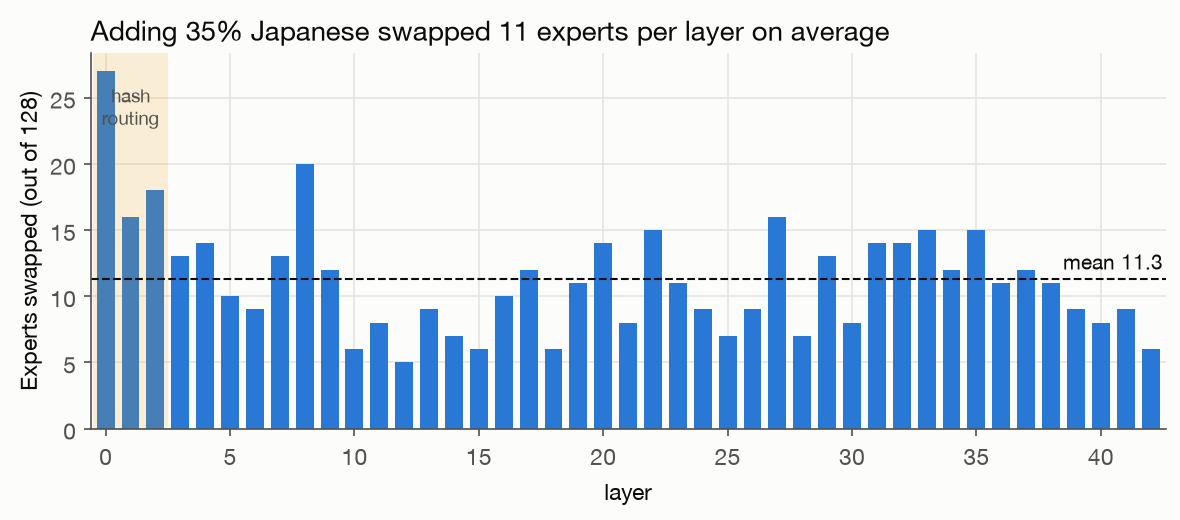
11 out of 128. That alone brought Japanese back. The answers to the same questions became:
Highest mountain: 日本で一番高い山は富士山(ふじさん)で、標高は3,776メートルです。 Correct, and in Japanese: Mount Fuji, 3,776 meters.
Miso soup: a sane four-step recipe in Japanese: make dashi, cut the vegetables, simmer them, dissolve the miso. One glitch: in step 4, 味噌 (miso) is rendered as 味噰.
Haiku: 秋の風やけしの実の音やまず / 季語:秋の風 The autumn wind, the rattle of dry poppy pods; seasonal word: autumn wind. In the commentary line, the 詠 of 詠みました (composed) is rendered as �.
The miso soup recipe is back to sanity. The two glitches, 味噰 and �, are a remaining side effect, covered in section 6.
If you run this pipeline for another language, be sure to include that language in the mix. Using the REAP paper’s setup as-is removes everything that is not English.
4. Challenge 2: architectural walls specific to DeepSeek-V4
“Delete experts and remove the corresponding router rows” is not enough for V4 to work. There are four structures specific to V4.
(1) Hash routing in layers 0 to 2 (tid2eid)
The first 3 layers of V4 do not have a learned router. They route through a fixed table gate.tid2eid (shape [vocab_size, 6]) that maps token IDs to experts. This is why layer 1 in the cumulative share figure in section 2 had a nearly uniform distribution.
If you delete experts here, the table is left with expert IDs that no longer exist. Tokens that were assigned to deleted experts have to be reassigned somewhere.
The approach I took was to reassign to the closest surviving expert by cosine similarity of the router rows (each row of gate.weight is a 4096-dimensional vector per expert). The 6 experts for a token must not contain duplicates, so candidates are scanned in similarity order and the first unused one is chosen.
sim = normalize(gate_weight) @ normalize(gate_weight[keep]).T   # [256, 128]
ranked = keep[argsort(sim, descending=True)]                    # replacement candidates per expert, closest first
for row in table[rows_with_removed_ids]:
    used = {e for e in row if is_kept[e]}
    for j, e in enumerate(row):
        if not is_kept[e]:
            row[j] = next(c for c in ranked[e] if c not in used); used.add(row[j])
Since the hash layers do not select by router weights in the first place, “similar router row = similar function” is a heuristic. But the layer with the most swaps (27) in the Japanese recalibration was layer 0, so the experts in the hash layers are clearly corpus-dependent too, and selecting them by REAP score is meaningful.
(2) Slicing the router bias (gate.bias / noaux_tc) in sync
V4’s router uses the same auxiliary-loss-free load balancing as the DeepSeek-V3 family and holds a per-expert correction bias in gate.bias. Top-k selection uses the score with the bias added, and the output weights use the score without it: a two-stage design.
When pruning, the rows of gate.weight and the elements of gate.bias are sliced with the same keep index. Misalign them and the experts being selected and the experts being weighted become different things, and the model breaks silently.
entries.append(tensor_to_entry(name, reader.tensor(name).index_select(0, keep), info["dtype"]))(3) Detaching MTP (Multi-Token Prediction)
V4 Flash ships with an MTP head mtp.0.* for speculative decoding, which has its own independent set of 256 experts. I dropped it entirely and set num_nextn_predict_layers in config.json to 0.
Two reasons. Keeping MTP would mean pruning its experts too so the sizes match, which needs another stage of the calibration pipeline. And I could not estimate the cost of verifying that vLLM’s MTP speculative decoding works correctly on a pruned V4. As a proof of concept, getting the main body running came first. This costs decode speed, discussed in section 7.
(4) vLLM’s kernel constraint (K=128 and 192 are native)
vLLM’s DeepSeek-V4 implementation computes the router’s top-k with a fused kernel called topk_softplus_sqrt. This kernel supports only specific expert counts: 16, 32, 64, 128, 192, 256, and so on.
Looking at size alone, K=160 (101 GB) is attractive. 0xSero’s previously published 180B version uses K=160 and runs with a router fallback patch applied to vLLM. This time I prioritized “runs on stock vLLM” and chose K=128. K=192 (119 GB) does fit, but leaves less than 10 GB for the KV cache, which is not practical.
5. Challenge 3: slicing FP4/FP8 weights byte by byte without requantizing
Decoding and requantizing degrades quality and takes time
When writing out the pruned checkpoint, the naive approach is “convert everything to bf16, remove the unwanted experts, quantize back to FP4/FP8”. This loses in two ways.
- FP4 block quantization has freedom in how scales are chosen, and there is no guarantee of reproducing the quantization DeepSeek used for distribution. The round trip adds error
- Dequantizing and requantizing 167 GB takes time. And the Spark has nowhere to put it
More fundamentally, not a single byte of the kept experts’ weights changes, so there is no need to convert anything.
Copy the safetensors bytes directly and regenerate the header
safetensors is a simple format: the first 8 bytes are the header length, followed by a JSON header, followed by the raw tensor data. The header only records each tensor’s dtype, shape, and data_offsets (start and end within the data region).
So pruning reduces to “read the header, decide what to do with each tensor, lay the raw bytes out in a new file, and rewrite the header”.
| Tensor | Action |
|---|---|
layers.N.ffn.experts.E.* (E in keep) |
Renumber E to the new sequential index and copy the raw bytes as-is |
layers.N.ffn.experts.E.* (E not in keep) |
Drop |
layers.N.ffn.gate.weight / gate.bias |
index_select the kept rows and rewrite (the only real bf16/fp32 tensor operation) |
layers.N.ffn.gate.tid2eid (hash layers) |
Write the table reassigned in section 4 (1), renumbered to the new indices |
mtp.* |
Drop |
| Everything else (attention, embeddings, norms, …) | Copy the raw bytes as-is |
def write_shard(path, tensors):
    header, offset = {"__metadata__": {"format": "pt"}}, 0
    for name, dtype, shape, data in tensors:
        header[name] = {"dtype": dtype, "shape": shape, "data_offsets": [offset, offset + len(data)]}
        offset += len(data)
    hjson = json.dumps(header, separators=(",", ":")).encode()
    hjson += b" " * (-len(hjson) % 8)
    with open(path, "wb") as f:
        f.write(struct.pack("<Q", len(hjson))); f.write(hjson)
        for *_, data in tensors:
            f.write(data)
The process is dominated by disk I/O and uses neither the GPU nor much memory. After writing 45 shards, 34,588 tensors, 82.4 GB, a separate header-level validation runs: consistency between the index and each shard, whether every layer has experts 0 to 127 without gaps and with matching w1/w2/w3 weights and scales, whether any mtp.* remains, and so on.
As a by-product, reading just the headers of the original checkpoint via HTTP Range requests gives you the tensor list and a size estimate without downloading anything. The size chart in section 1 was produced that way.
6. Serving and benchmark results
Getting it running on vLLM
Install vLLM 0.28.0 with pip and it starts as-is.
vllm serve ludo-tech/DeepSeek-V4-Flash-REAP-145B-A13B \
  --served-model-name v4-flash-k128 \
  --max-model-len 32768 \
  --gpu-memory-utilization 0.80 \
  --kv-cache-dtype fp8
There were three Spark-specific pitfalls.
--kv-cache-dtype fp8is required. V4’s attention assumes the fp8 MLA KV layout- The Spark has no nvcc. Since FlashInfer kernels cannot be built, install
flashinfer-cubinandflashinfer-jit-cacheseparately, at the same version as the flashinfer-python that vLLM installed. Forget this and vLLM silently falls back as if FlashInfer were absent. It still runs, just slowly, which makes it nasty to notice - V4 does not use a Jinja chat template. It goes through a dedicated encoder built into vLLM and defaults to thinking mode. To turn it off, add
--default-chat-template-kwargs '{"enable_thinking": false}'
Here is the output of the first warm-up request I sent before knowing about that last point.
Q: 1+1は? (What is 1+1?)
We need answer. User asks “1+1は?” likely Japanese? “1+1 is?” Need respond. Simple arithmetic. But must be careful: “1+1は?” maybe asking “what is 1+1” in Japanese. Answer: 2. …
The model is fine. It is just leaking its thinking.
Memory and speed
With --gpu-memory-utilization 0.80, handing 80 percent of 128 GB to vLLM, the 82 GB of weights fit alongside an fp8 KV cache for 32K context. MemAvailable during the benchmark stayed stable around 16 GB, enough headroom to load a small model in the co-resident ollama.
Results from generating 57 prompts back to back:
| Metric | Value |
|---|---|
| Decode speed (median / min / max) | 17.1 / 17.1 / 17.6 tok/s |
| TTFT (median) | 0.35 s |
| Failures / empty outputs | 0 / 0 |
This is reasonable for pushing 13B active parameters through the Spark’s 273 GB/s of bandwidth, and it is comfortably practical for chat. Since MTP was dropped, it is certainly slower than a configuration with speculative decoding.
Quality evaluation
This is a small in-house eval, not a benchmark suite. Code is checked by running the Python and testing it, math by numeric match, and Japanese by whether the answer is in Japanese including kana.
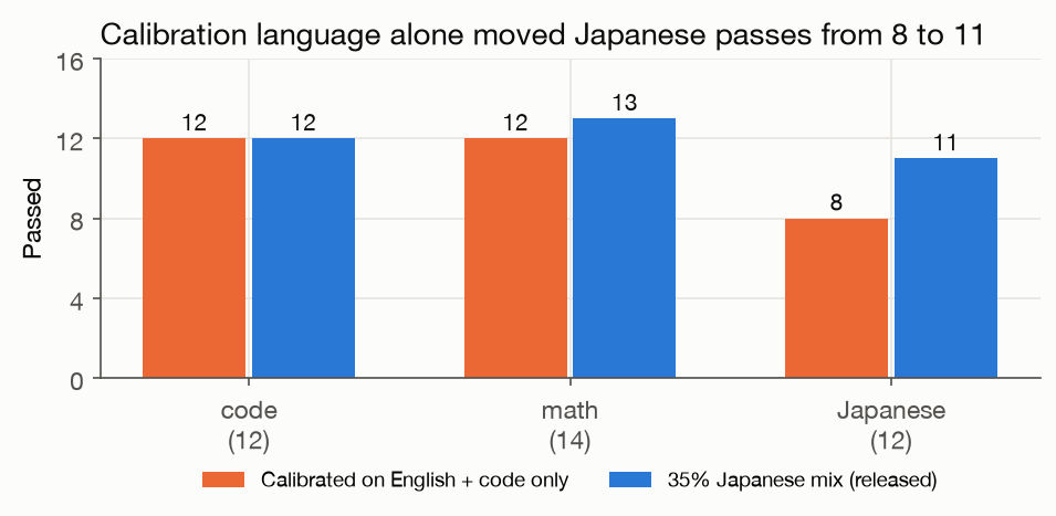
| Category | Items | Calibrated on English only | 35% Japanese mix (released) |
|---|---|---|---|
| code | 12 | 12 | 12 |
| math | 14 | 12 | 13 |
| Japanese | 12 | 8 | 11 |
The jump from 8 to 11 in Japanese is the effect of the recalibration in section 3. The English-only version’s 8 only passed the “output contains kana” check; the content was mixed with Chinese, as seen in section 3. Code and math did not drop from mixing in Japanese.
The one item the released version failed was “translate ‘this product goes on sale next month’ into English”. It translated correctly, which failed the kana check. That is a grading problem.
A remaining side effect: rare kanji drop out
Section 3’s outputs contained 味噰 and �みました. Even in the released version, a rare kanji occasionally drops out of the middle of a word or turns into a different character.
V4’s tokenizer is byte-level BPE, so low-frequency kanji become multi-byte token sequences. My reading is that the experts handling those byte sequences ranked low on REAP score and were dropped. Grammar and context are preserved. Including 20 percent Japanese Wikipedia rescued the frequently occurring kanji but did not reach the long tail. Raising the Japanese ratio further or adding a kanji-heavy corpus should help, but it is a trade-off against English and code.
Actual generation examples
A few outputs from the released version, summarized.
- Explain the difference between 了解しました and 承知いたしました (two ways to say “understood”). A structured answer: both acknowledge an instruction, 了解しました is flatter and more casual, 承知いたしました is the humble form for superiors and clients. Correct and idiomatic.
- Explain photosynthesis so that an elementary school student can understand. Plain, friendly Japanese: plants use sunlight, water, and air to make their own food, which comes out as starch and sugar.
- Write a polite email telling your manager you are taking a sick day. A properly formatted business email with subject line, addressee, and honorifics. One line reads 心よりお�び申し上げます, where the 詫 of 詫び (apology) has dropped out.
That お�び is the kanji dropout described above. 詫 is an everyday word, but as a byte sequence it appears to be low frequency.
7. Discussion and future work
The trade-off in the number of experts K
| K | Size | Stock vLLM | KV headroom (128 GB, util 0.80) | Outlook |
|---|---|---|---|---|
| 128 | 82 GB | Works | About 20 GB | This release |
| 160 | 101 GB | Needs a patch | About 1 GB | Quality should be higher, but practical use needs a higher util |
| 192 | 119 GB | Works | Does not fit | Not viable |
K=160 has 0xSero’s track record and is attractive on quality. But securing 32K context on a single Spark is a stretch: you would have to raise --gpu-memory-utilization to 0.9 or above and squeeze the OS. For “run it comfortably on one machine”, I think K=128 is the right compromise.
Varying K per layer (more in shallow layers, fewer in deep layers, or the reverse) is a natural extension. The cumulative share plot in section 2 shows that skew differs by layer, so a better allocation than a flat 128 should exist. But vLLM’s kernel constraint binds per-layer K to 128 or 192 as well, so there is currently no freedom there.
Left undone
- Restoring MTP. Applying the same REAP to the MTP head’s 256 experts and cutting them to 128 should bring back speculative decoding and raise decode speed
- Chinese. It was not in the calibration set, so what happened to Japanese in the English-only version very likely happened to Chinese here
- A proper benchmark. This eval is 38 items. That is not enough to quantify the gap from the original model
- Comparison against the DeepSeek API. Sending the same eval to the official API to see how many the original model passes is the smallest next step
Summary
- MoE pruning is a realistic way to fit a model that is already FP4/FP8, with no room for quantization, onto one machine. The kept tensors are copied byte for byte, so there is no requantization loss and no requantization time
- Even on a machine that cannot hold the full model, calibration is possible with layer streaming. All you need is GPU memory for one layer and an NVMe to hold the hidden states
- Selecting by contribution (REAP) rather than count changes 40 percent of the surviving experts
- The language of the calibration corpus decides which experts survive. If you need Japanese, put Japanese in. That alone swapped 11 experts per layer and turned a model that answered in Chinese into one that answers in Japanese
The full pipeline (inventory, calibration, plan, rewrite, validate) is in the tools/ directory of the Hugging Face repository. If you have a Spark, give it a try.
References
- REAP: Why Pruning Prevails for One-Shot MoE Compression (Cerebras) https://arxiv.org/abs/2510.13999
- DeepSeek-V4-Flash-0731 https://huggingface.co/deepseek-ai/DeepSeek-V4-Flash-0731
- 0xSero/DeepSeek-V4-Flash-180B (K=160, with vLLM patch) https://huggingface.co/0xSero/DeepSeek-V4-Flash-180B
- sleepyeldrazi/ds4-nvfp4-spark https://github.com/sleepyeldrazi/ds4-nvfp4-spark